Homeworks
These are some of the homework assignments I have completed during my Fall 2024 semester in CFD.

This assignment focused on vector calculus applications in fluid dynamics, involving gradient, Laplacian, and stress tensor calculations for incompressible flows. I calculated gradients and Laplacians of scalar functions, calcylated viscous stress tensors, and developed an expression for the pressure gradient.
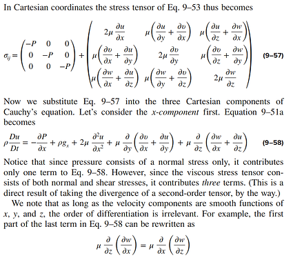
Çengel, Y. A., & Cimbala, J. M. (2018). Fluid mechanics : fundamentals and applications (4th ed., p. 473). Mcgraw-Hill Education.
Homework 1
This assignment involved deriving a second-order accurate estimate for the first derivative using polynomial fitting on a uniform grid. Additionally, I analyzed the limitations of the uniform grid, observing that an 11-point grid failed to accurately capture regions with rapidly changing gradients. To address this, I designed a refined grid with an appropriate expansion factor to better resolve gradients across the domain.

Coarse grid and refined grid approximations for solving the provided derivative.
Homework 2
In this assignment, I was tasked with solving the 1D convection-diffusion problem by applying the central difference scheme to both the convective and diffusion terms. I varied the grid points and Peclet number to analyze their effects on solution accuracy. Following this, I implemented the backward difference scheme for the convective term while retaining the central difference scheme for the diffusion term, allowing for a comparison of the schemes under different configurations.

Exact solution (solid line) compared to the CDS numerical solution (dashed line) of the PDE using Pe=12.5 and n=25.
Homework 3
In this assignment, I developed code to solve a linear system of equations using the Gauss-Seidel method, with functionality to handle no-relaxation, under-relaxation, and over-relaxation scenarios. Given two A matrices and corresponding b vector, I calculated the condition numbers of each matrix to predict which system would converge more quickly. I then solved for the ϕ solution vector for each system and determined the optimal relaxation factor for enhanced convergence in both cases.

(a) On the left, graphical representation of the residual vs the number of iterations for matrix A2 when gamma equals 0.5 (no convergence). (b) In the middle, graphical representation of the residual vs the number of iterations for matrix A2 when gamma equals 1.81 (converged in 97 iterations).
Homework 4 (Part 1)
In this assignment, I investigated how error decay in numerical solutions depends on grid resolution relative to error wavelength. Using the Gauss-Seidel iterative method, I solved a steady-state, one-dimensional heat conduction problem with given boundary conditions and an initial temperature distribution containing both high- and low-frequency error components. I plotted the solution, along with the maximum error and residual across the domain, over various iterations to visualize how the grid resolution influences error decay for different error wavelengths.

Residuals calculated as the absolute difference between the two consecutive iterations of T over each position x. Iterations chosen by user to show effect of residual at each iteration.